3 Efficient programming

Many people who use R would not describe themselves as “programmers”. Instead they tend to have advanced domain level knowledge, understand standard R data structures, such as vectors and data frames, but have little formal training in computing. Sound familiar? In that case this chapter is for you.

In this chapter we will discuss “big picture” programming techniques. We cover general concepts and R programming techniques about code optimisation, before describing idiomatic programming structures. We conclude the chapter by examining relatively easy ways of speeding up code using the compiler package and parallel processing, using multiple CPUs.

Prerequisites

In this chapter we introduce two new packages, compiler and memoise. The compiler package comes with R, so it will already be installed.

library("compiler")
library("memoise")

We also use the pryr and microbenchmark packages in the exercises.

3.1 Top 5 tips for efficient programming

Be careful never to grow vectors.
Vectorise code whenever possible.
Use factors when appropriate.
Avoid unnecessary computation by caching variables.
Byte compile packages for an easy performance boost.

3.2 General advice

Low level languages like C and Fortran demand more from the programmer. They force you to declare the type of every variable used, give you the burdensome responsibility of memory management and have to be compiled. The advantage of such languages, compared with R, is that they are faster to run. The disadvantage is that they take longer to learn and can not be run interactively.

The Wikipedia page on compiler optimisations gives a nice overview of standard optimisation techniques (https://en.wikipedia.org/wiki/Optimizing_compiler).

R users don’t tend to worry about data types. This is advantageous in terms of creating concise code, but can result in R programs that are slow. While optimisations such as going parallel can double speed, poor code can easily run hundreds of times slower, so it’s important to understand the causes of slow code. These are covered in Burns (2011), which should be considered essential reading for any aspiring R programmers.

Ultimately calling an R function always ends up calling some underlying C/Fortran code. For example the base R function runif() only contains a single line that consists of a call to C_runif().

function(n, min = 0, max = 1)
  .Call(C_runif, n, min, max)

A golden rule in R programming is to access the underlying C/Fortran routines as quickly as possible; the fewer functions calls required to achieve this, the better. For example, suppose x is a standard vector of length n. Then

x = x + 1

involves a single function call to the + function. Whereas the for loop

for (i in seq_len(n))
  x[i] = x[i] + 1

has

n function calls to +;
n function calls to the [ function;
n function calls to the [<- function (used in the assignment operation);
Two function calls: one to for and another to seq_len().

It isn’t that the for loop is slow, rather it is because we have many more function calls. Each individual function call is quick, but the total combination is slow.

Everything in R is a function call. When we execute 1 + 1, we are actually executing ‘+’(1, 1).

Exercise

Use the microbenchmark package to compare the vectorised construct x = x + 1, to the for loop version. Try varying the size of the input vector.

3.2.1 Memory allocation

Another general technique is to be careful with memory allocation. If possible pre-allocate your vector then fill in the values.

You should also consider pre-allocating memory for data frames and lists. Never grow an object. A good rule of thumb is to compare your objects before and after a for loop; have they increased in length?

Let’s consider three methods of creating a sequence of numbers. Method 1 creates an empty vector and gradually increases (or grows) the length of the vector:

method1 = function(n) {
  vec = NULL # Or vec = c()
  for (i in seq_len(n))
    vec = c(vec, i)
  vec
}

Method 2 creates an object of the final length and then changes the values in the object by subscripting:

method2 = function(n) {
  vec = numeric(n)
  for (i in seq_len(n))
    vec[i] = i
  vec
}

Method 3 directly creates the final object:

method3 = function(n) seq_len(n)

To compare the three methods we use the microbenchmark() function from the previous chapter

microbenchmark(times = 100, unit = "s",
               method1(n), method2(n), method3(n))

The table below shows the timing in seconds on my machine for these three methods for a selection of values of n. The relationships for varying n are all roughly linear on a log-log scale, but the timings between methods are drastically different. Notice that the timings are no longer trivial. When \(n=10^7\), Method 1 takes around an hour whilst Method 2 takes \(2\) seconds and Method 3 is almost instantaneous. Remember the golden rule; access the underlying C/Fortran code as quickly as possible.

Time in seconds to create sequences. When \(n=10^7\), Method 1 takes around an hour while the other methods take less than \(3\) seconds.
\(n\)	Method 1	Method 2	Method 3
\(10^5\)	\(\phantom{000}0.21\)	\(0.02\)	\(0.00\)
\(10^6\)	\(\phantom{00}25.50\)	\(0.22\)	\(0.00\)
\(10^7\)	\(3827.00\)	\(2.21\)	\(0.00\)

3.2.2 Vectorised code

Technically x = 1 creates a vector of length \(1\). In this section, we use vectorised to indicate that functions work with vectors of all lengths.

Recall the golden rule in R programming, access the underlying C/Fortran routines as quickly as possible; the fewer functions calls required to achieve this, the better. With this mind, many R functions are vectorised, that is the function’s inputs and/or outputs naturally work with vectors, reducing the number of function calls required. For example, the code

x = runif(n) + 1

performs two vectorised operations. First runif() returns n random numbers. Second we add 1 to each element of the vector. In general it is a good idea to exploit vectorised functions. Consider this piece of R code that calculates the sum of \(\log(x)\)

log_sum = 0
for (i in 1:length(x))
  log_sum = log_sum + log(x[i])

Using 1:length(x) can lead to hard-to-find bugs when x has length zero. Instead use seq_along(x) or seq_len(length(x)).

This code could easily be vectorised via

log_sum = sum(log(x))

Writing code this way has a number of benefits.

It’s faster. When \(n = 10^7\) the R way is about forty times faster.
It’s neater.
It doesn’t contain a bug when x is of length \(0\).

As with the general example in Section 3.2, the slowdown isn’t due to the for loop. Instead, it’s because there are many more function calls.

Exercises

Time the two methods for calculating the log sum.
What happens when the length(x) = 0, i.e. we have an empty vector?

Example: Monte-Carlo integration

It’s also important to make full use of R functions that use vectors. For example, suppose we wish to estimate the integral \[ \int_0^1 x^2 dx \] using a Monte-Carlo method. Essentially, we throw darts at the curve and count the number of darts that fall below the curve (as in 3.1).

Monte Carlo Integration

Initialise: hits = 0
for i in 1:N
\(~~~\) Generate two random numbers, \(U_1, U_2\), between 0 and 1
\(~~~\) If \(U_2 < U_1^2\), then hits = hits + 1
end for
Area estimate = hits/N

Implementing this Monte-Carlo algorithm in R would typically lead to something like:

monte_carlo = function(N) {
  hits = 0
  for (i in seq_len(N)) {
    u1 = runif(1)
    u2 = runif(1)
    if (u1 ^ 2 > u2)
      hits = hits + 1
  }
  return(hits / N)
}

In R, this takes a few seconds

N = 500000
system.time(monte_carlo(N))
#>    user  system elapsed 
#>   2.206   0.004   2.210

In contrast, a more R-centric approach would be

monte_carlo_vec = function(N) sum(runif(N)^2 > runif(N)) / N

The monte_carlo_vec() function contains (at least) four aspects of vectorisation

The runif() function call is now fully vectorised;
We raise entire vectors to a power via ^;
Comparisons using > are vectorised;
Using sum() is quicker than an equivalent for loop.

The function monte_carlo_vec() is around \(30\) times faster than monte_carlo().

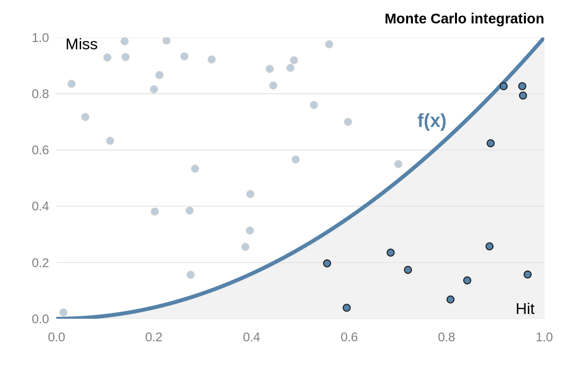
Example of Monte-Carlo integration. To estimate the area under the curve, throw random points at the graph and count the number of points that lie under the curve.

Figure 3.1: Example of Monte-Carlo integration. To estimate the area under the curve, throw random points at the graph and count the number of points that lie under the curve.

Exercise

Verify that monte_carlo_vec() is faster than monte_carlo(). How does this relate to the number of darts, i.e. the size of N, that is used?

3.3 Communicating with the user

When we create a function we often want the function to give efficient feedback on the current state. For example, are there missing arguments or has a numerical calculation failed. There are three main techniques for communicating with the user.

Fatal errors: `stop()`

Fatal errors are raised by calling the stop(), i.e. execution is terminated. When stop() is called, there is no way for a function to continue. For instance, when we generate random numbers using rnorm() the first argument is the sample size,n. If the number of observations to return is less than \(1\), an error is raised. When we need to raise an error, we should do so as quickly as possible; otherwise it’s a waste of resources. Hence, the first few lines of a function typically perform argument checking.

Suppose we call a function that raises an error. What then? Efficient, robust code catches the error and handles it appropriately. Errors can be caught using try() and tryCatch(). For example,

# Suppress the error message
good = try(1 + 1, silent = TRUE)
bad = try(1 + "1", silent = TRUE)

When we inspect the objects, the variable good just contains the number 2

good
#> [1] 2

However, the bad object is a character string with class try-error and a condition attribute that contains the error message

bad
#> [1] "Error in 1 + \"1\" : non-numeric argument to binary operator\n"
#> attr(,"class")
#> [1] "try-error"
#> attr(,"condition")
#> <simpleError in 1 + "1": non-numeric argument to binary operator>

We can use this information in a standard conditional statement

if (class(bad) == "try-error")
  # Do something

Further details on error handling, as well as some excellent advice on general debugging techniques, are given in H. Wickham (2014 a).

Warnings: `warning()`

Warnings are generated using the warning() function. When a warning is raised, it indicates potential problems. For example, mean(NULL) returns NA and also raises a warning.

When we come across a warning in our code, it is important to solve the problem and not just ignore the issue. While ignoring warnings saves time in the short-term, warnings can often mask deeper issues that have crept into our code.

Warnings can be hidden using suppressWarnings().

Informative output: `message()` and `cat()`

To give informative output, use the message() function. For example, in the poweRlaw package, the message() function is used to give the user an estimate of expected run time. Providing a rough estimate of how long the function takes, allows the user to optimise their time. Similar to warnings, messages can be suppressed with suppressMessages().

Another function used for printing messages is cat(). In general cat() should only be used in print()/show() methods, e.g. look at the function definition of the S3 print method for difftime objects, getS3method("print", "difftime").

Exercises

The stop() function has an argument call. that indicates if the function call should be part of the error message. Create a function and experiment with this option.

3.3.1 Invisible returns

The invisible() function allows you to return a temporarily invisible copy of an object. This is particularly useful for functions that return values which can be assigned, but are not printed when they are not assigned. For example suppose we have a function that plots the data and fits a straight line

regression_plot = function(x, y, ...) {
  # Plot and pass additional arguments to default plot method
  plot(x, y, ...)

  # Fit regression model
  model = lm(y ~ x)

  # Add line of best fit to the plot
  abline(model)
  invisible(model)
}

When the function is called, a scatter graph is plotted with the line of best fit, but the output is invisible. However when we assign the function to an object, i.e. out = regression_plot(x, y) the variable out contains the output of the lm() call.

Another example is the histogram function hist(). Typically we don’t want anything displayed in the console when we call the function

hist(x)

However if we assign the output to an object, out = hist(x), the object out is actually a list containing, inter alia, information on the mid-points, breaks and counts.

3.4 Factors

Factors are much maligned objects. While at times they are awkward, they do have their uses. A factor is used to store categorical variables. This data type is unique to R (or at least not common among programming languages). The difference between factors and strings is important because R treats factors and strings differently. Although factors look similar to character vectors, they are actually integers. This leads to initially surprising behaviour

x = 4:6
c(x)
#> [1] 4 5 6
c(factor(x))
#> [1] 1 2 3

In this case the c() function is using the underlying integer representation of the factor. Dealing with the wrong case of behaviour is a common source of inefficiency for R users.

Often categorical variables get stored as \(1\), \(2\), \(3\), \(4\), and \(5\), with associated documentation elsewhere that explains what each number means. This is clearly a pain. Alternatively we store the data as a character vector. While this is fine, the semantics are wrong because it doesn’t convey that this is a categorical variable. It’s not sensible to say that you should always or never use factors, since factors have both positive and negative features. Instead we need to examine each case individually.

As a general rule, if your variable has an inherent order, e.g. small vs large, or you have a fixed set of categories, then you should consider using a factor.

3.4.1 Inherent order

Factors can be used for ordering in graphics. For instance, suppose we have a data set where the variable type, takes one of three values, small, medium and large. Clearly there is an ordering. Using a standard boxplot() call,

boxplot(y ~ type)

would create a boxplot where the \(x\)-axis was alphabetically ordered. By converting type into factor, we can easily specify the correct ordering.

boxplot(y ~ factor(type, levels = c("Small", "Medium", "Large")))

Most users interact with factors via the read.csv() function where character columns are automatically converted to factors. This feature can be irritating if our data is messy and we want to clean and recode variables. Typically when reading in data via read.csv(), we use the stringsAsFactors = FALSE argument. Although this argument can be added to the global options() list and placed in the .Rprofile, this leads to non-portable code, so should be avoided.

3.4.2 Fixed set of categories

Suppose our data set relates to months of the year

m = c("January", "December", "March")

If we sort m in the usual way, sort(m), we perform standard alpha-numeric ordering; placing December first. This is technically correct, but not that helpful. We can use factors to remedy this problem by specifying the admissible levels

# month.name contains the 12 months
fac_m = factor(m, levels = month.name)
sort(fac_m)
#> [1] January  March    December
#> 12 Levels: January February March April May June July August ... December

Exercise

Factors are slightly more space efficient than characters. Create a character vector and corresponding factor and use pryr::object_size() to calculate the space needed for each object.

3.5 The apply family

The apply functions can be an alternative to writing for loops. The general idea is to apply (or map) a function to each element of an object. For example, you can apply a function to each row or column of a matrix. A list of available functions is given in Table 3.1, with a short description. In general, all the apply functions have similar properties:

Each function takes at least two arguments: an object and another function. The function is passed as an argument.
Every apply function has the dots, ..., argument that is used to pass on arguments to the function that is given as an argument.

Using apply functions when possible, can lead to more succinct and idiomatic R code. In this section, we will cover the three main functions, apply(), lapply(), and sapply(). Since the apply functions are covered in most R textbooks, we just give a brief introduction to the topic and provide pointers to other resources at the end of this section.

Most people rarely use the other apply functions. For example, I have only used eapply() once. Students in my class uploaded R scripts. Using source(), I was able to read in the scripts to a separate environment. I then applied a marking scheme to each environment using eapply(). Using separate environments, avoided object name clashes.

Table 3.1: The apply family of functions from base R.
Function	Description
`apply`	Apply functions over array margins
`by`	Apply a function to a data frame split by factors
`eapply`	Apply a function over values in an environment
`lapply`	Apply a function over a list or vector
`mapply`	Apply a function to multiple list or vector arguments
`rapply`	Recursively apply a function to a list
`tapply`	Apply a function over a ragged array

The apply() function is used to apply a function to each row or column of a matrix. In many data science problems, this is a common task. For example, to calculate the standard deviation of the rows we have

data("ex_mat", package = "efficient")
# MARGIN=1: corresponds to rows
row_sd = apply(ex_mat, 1, sd)

The first argument of apply() is the object of interest. The second argument is the MARGIN. This is a vector giving the subscripts which the function (the third argument) will be applied over. When the object is a matrix, a margin of 1 indicates rows and 2 indicates columns. So to calculate the column standard deviations, the second argument is changed to 2

col_sd = apply(ex_mat, 2, sd)

Additional arguments can be passed to the function that is to be applied to the data. For example, to pass the na.rm argument to the sd function, we have

row_sd = apply(ex_mat, 1, sd, na.rm = TRUE)

The apply() function also works on higher dimensional arrays; a one dimensional array is a vector, a two dimensional array is a matrix.

The lapply() function is similar to apply(); with the key difference being that the input type is a vector or list and the return type is a list. Essentially, we apply a function to each element of a list or vector. The functions sapply() and vapply() are similar to lapply(), but the return type is not necessary a list.

3.5.1 Example: the movies data set

The Internet Movie Database is a website that collects movie data supplied by studios and fans. It is one of the largest movie databases on the web and is maintained by Amazon. The ggplot2movies package contains about sixty thousand movies stored as a data frame

data(movies, package = "ggplot2movies")

Movies are rated between \(1\) and \(10\) by fans. Columns \(7\) to \(16\) of the movies data set gives the percentage of voters for a particular rating.

ratings = movies[, 7:16]

For example, 4.5% of voters, rated the first movie a rating of \(1\)

ratings[1, ]
#> # A tibble: 1 x 10
#>      r1    r2    r3    r4    r5    r6    r7    r8    r9   r10
#>   <dbl> <dbl> <dbl> <dbl> <dbl> <dbl> <dbl> <dbl> <dbl> <dbl>
#> 1   4.5   4.5   4.5   4.5  14.5  24.5  24.5  14.5   4.5   4.5

We can use the apply() function to investigate voting patterns. The function nnet::which.is.max() finds the maximum position in a vector, but breaks ties at random; which.max() just returns the first value. Using apply(), we can easily determine the most popular rating for each movie and plot the results

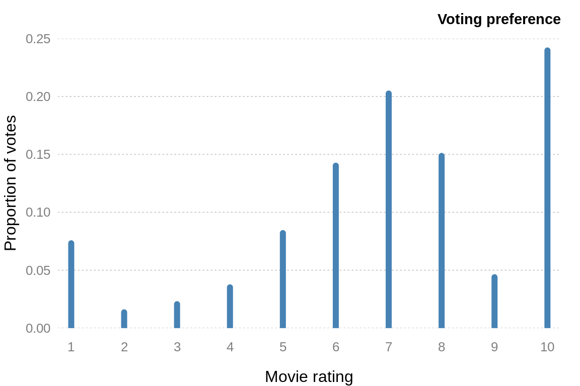
popular = apply(ratings, 1, nnet::which.is.max)
plot(table(popular))

Figure 3.2: Movie voting preferences.

Figure 3.2 highlights that voting patterns are clearly not uniform between \(1\) and \(10\). The most popular vote is the highest rating, \(10\). Clearly if you went to the trouble of voting for a movie, it was either very good, or very bad (there is also a peak at \(1\)). Rating a movie \(7\) is also a popular choice (search the web for “most popular number” and \(7\) dominates the rankings).

3.5.2 Type consistency

When programming, it is helpful if the return value from a function always takes the same form. Unfortunately, not all base R functions follow this idiom. For example, the functions sapply() and [.data.frame() aren’t type consistent

two_cols = data.frame(x = 1:5, y = letters[1:5])
zero_cols = data.frame()
sapply(two_cols, class)  # a character vector
sapply(zero_cols, class) # a list
two_cols[, 1:2]          # a data.frame
two_cols[, 1]            # an integer vector

This can cause unexpected problems. The functions lapply() and vapply() are type consistent. Likewise for dplyr::select() and dplyr:filter(). The purrr package has some type consistent alternatives to base R functions. For example, map_dbl() (and other map_* functions) to replace Map() and flatten_df() to replace unlist().

Other resources

Almost every R book has a section on the apply function. Below, we’ve given the resources we feel are most helpful.

Each function has a number of examples in the associated help page. You can directly access the examples using the example() function, e.g. to run the apply() examples, use example("apply").
There is a very detailed StackOverflow answer which describes when, where and how to use each of the functions.
In a similar vein, Neil Saunders has a nice blog post giving an overview of the functions.
The apply functions are an example of functional programming. Chapter 16 of R for Data Science (Grolemund and Wickham 2016) describes the interplay between loops and functional programming in more detail, while H. Wickham (2014 a) gives a more in-depth description of the topic.

Exercises

Rewrite the sapply() function calls above using vapply() to ensure type consistency.
How would you make subsetting data frames with [ type consistent? Hint: look at the drop argument.

3.6 Caching variables

A straightforward method for speeding up code is to calculate objects once and reuse the value when necessary. This could be as simple as replacing sd(x) in multiple function calls with the object sd_x that is defined once and reused. For example, suppose we wish to normalise each column of a matrix. However, instead of using the standard deviation of each column, we will use the standard deviation of the entire data set

apply(x, 2, function(i) mean(i) / sd(x))

This is inefficient since the value of sd(x) is constant and thus recalculating the standard deviation for every column is unnecessary. Instead we should evaluate once and store the result

sd_x = sd(x)
apply(x, 2, function(i) mean(i) / sd_x)

If we compare the two methods on a \(100\) row by \(1000\) column matrix, the cached version is around \(100\) times faster (Figure 3.3).

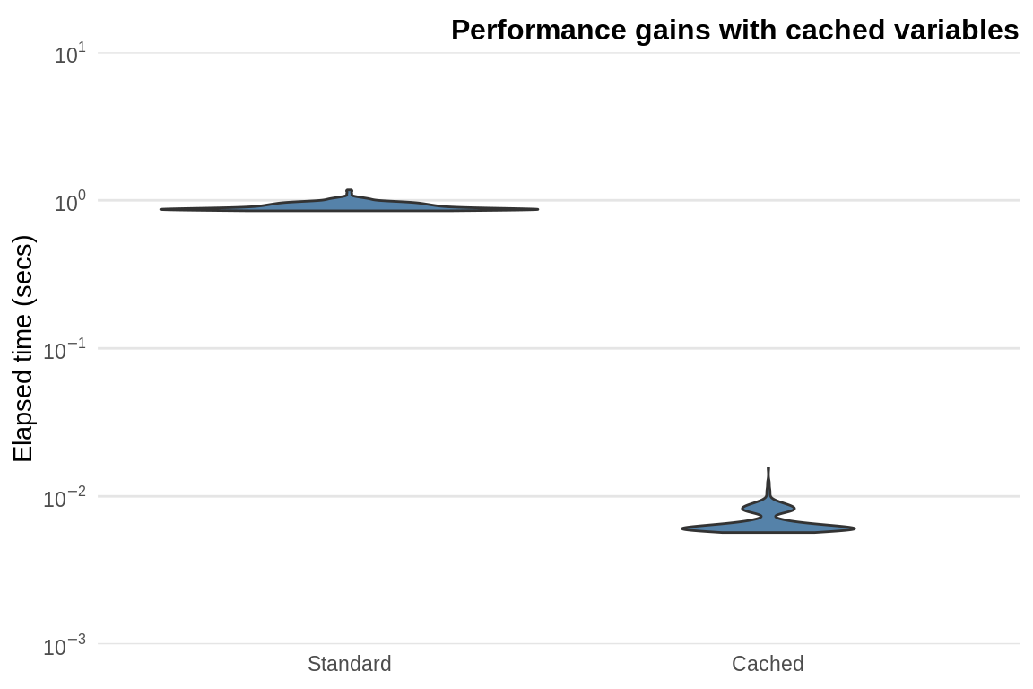
Figure 3.3: Performance gains obtained from caching the standard deviation in a \(100\) by \(1000\) matrix.

A more advanced form of caching is to use the memoise package. If a function is called multiple times with the same input, it may be possible to speed things up by keeping a cache of known answers that it can retrieve. The memoise package allows us to easily store the value of function call and returns the cached result when the function is called again with the same arguments. This package trades off memory versus speed, since the memoised function stores all previous inputs and outputs. To cache a function, we simply pass the function to the memoise function.

The classic memoise example is the factorial function. Another example is to limit use to a web resource. For example, suppose we are developing a Shiny (an interactive graphic) application where the user can fit a regression line to data. The user can remove points and refit the line. An example function would be

# Argument indicates row to remove
plot_mpg = function(row_to_remove) {
  data(mpg, package = "ggplot2")
  mpg = mpg[-row_to_remove, ]
  plot(mpg$cty, mpg$hwy)
  lines(lowess(mpg$cty, mpg$hwy), col = 2)
}

We can use memoise to speed up repeated function calls by caching results. A quick benchmark

m_plot_mpg = memoise(plot_mpg)
microbenchmark(times = 10, unit = "ms", m_plot_mpg(10), plot_mpg(10))
#> Unit: milliseconds
#>            expr   min    lq  mean median    uq   max neval cld
#>  m_plot_mpg(10)  0.04 4e-02  0.07  8e-02 8e-02   0.1    10  a
#>    plot_mpg(10) 40.20 1e+02 95.52  1e+02 1e+02 107.1    10   b

suggests that we can obtain a \(100\)-fold speed-up.

Exercise

Construct a box plot of timings for the standard plotting function and the memoised version.

3.6.1 Function closures

The following section is meant to provide an introduction to function closures with example use cases. See H. Wickham (2014 a) for a detailed introduction.

More advanced caching is available using function closures. A closure in R is an object that contains functions bound to the environment the closure was created in. Technically all functions in R have this property, but we use the term function closure to denote functions where the environment is not in .GlobalEnv. One of the environments associated with a function is known as the enclosing environment, that is, where the function was created. This allows us to store values between function calls. Suppose we want to create a stop-watch type function. This is easily achieved with a function closure

# <<- assigns values to the parent environment
stop_watch = function() {
  start_time = stop_time = NULL
  start = function() start_time <<- Sys.time()
  stop = function() {
    stop_time <<- Sys.time()
    difftime(stop_time, start_time)
  }
  list(start = start, stop = stop)
}
watch = stop_watch()

The object watch is a list, that contains two functions. One function for starting the timer

watch$start()

the other for stopping the timer

watch$stop()

Without using function closures, the stop-watch function would be longer, more complex and therefore more inefficient. When used properly, function closures are very useful programming tools for writing concise code.

Exercise

Write a stop-watch function without using function closures.
Many stop-watches have the ability to measure not only your overall time but also your individual laps. Add a lap() function to the stop_watch() function that will record individual times, while still keeping track of the overall time.

A related idea to function closures, is non-standard evaluation (NSE), or programming on the language. NSE crops up all the time in R. For example, when we execute plot(height, weight), R automatically labels the x- and y-axis of the plot with height and weight. This is a powerful concept that enables us to simplify code. More detail is given about “Non-standard evaluation” in H. Wickham (2014 a).

3.7 The byte compiler

The compiler package, written by R Core member Luke Tierney has been part of R since version 2.13.0. The compiler package allows R functions to be compiled, resulting in a byte code version that may run faster⁸. The compilation process eliminates a number of costly operations the interpreter has to perform, such as variable lookup.

Since R 2.14.0, all of the standard functions and packages in base R are pre-compiled into byte-code. This is illustrated by the base function mean():

getFunction("mean")
#> function (x, ...) 
#> UseMethod("mean")
#> <bytecode: 0x242e2c0>
#> <environment: namespace:base>

The third line contains the bytecode of the function. This means that the compiler package has translated the R function into another language that can be interpreted by a very fast interpreter. Amazingly the compiler package is almost entirely pure R, with just a few C support routines.

3.7.1 Example: the mean function

The compiler package comes with R, so we just need to load the package in the usual way

library("compiler")

Next we create an inefficient function for calculating the mean. This function takes in a vector, calculates the length and then updates the m variable.

mean_r = function(x) {
  m = 0
  n = length(x)
  for (i in seq_len(n))
    m = m + x[i] / n
  m
}

This is clearly a bad function and we should just use the mean() function, but it’s a useful comparison. Compiling the function is straightforward

cmp_mean_r = cmpfun(mean_r)

Then we use the microbenchmark() function to compare the three variants

# Generate some data
x = rnorm(1000)
microbenchmark(times = 10, unit = "ms", # milliseconds
          mean_r(x), cmp_mean_r(x), mean(x))
#> Unit: milliseconds
#>           expr   min    lq  mean median    uq  max neval cld
#>      mean_r(x) 0.358 0.361 0.370  0.363 0.367 0.43    10   c
#>  cmp_mean_r(x) 0.050 0.051 0.052  0.051 0.051 0.07    10  b
#>        mean(x) 0.005 0.005 0.008  0.007 0.008 0.03    10 a

The compiled function is around seven times faster than the uncompiled function. Of course the native mean() function is faster, but compiling does make a significant difference (Figure 3.4).

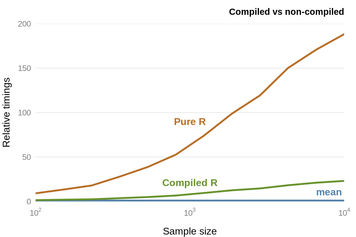
Figure 3.4: Comparison of mean functions.

3.7.2 Compiling code

There are a number of ways to compile code. The easiest is to compile individual functions using cmpfun(), but this obviously doesn’t scale. If you create a package, you can automatically compile the package on installation by adding

ByteCompile: true

to the DESCRIPTION file. Most R packages installed using install.packages() are not compiled. We can enable (or force) packages to be compiled by starting R with the environment variable R_COMPILE_PKGS set to a positive integer value and specify that we install the package from source, i.e.

## Windows users will need Rtools
install.packages("ggplot2", type = "source")

Or if we want to avoid altering the .Renviron file, we can specify an additional argument

install.packages("ggplot2", type = "source", INSTALL_opts = "--byte-compile")

A final option is to use just-in-time (JIT) compilation. The enableJIT() function disables JIT compilation if the argument is 0. Arguments 1, 2, or 3 implement different levels of optimisation. JIT can also be enabled by setting the environment variable R_ENABLE_JIT, to one of these values.

We recommend setting the compile level to the maximum value of 3.

The impact of compiling on install will vary from package to package: for packages that already have lots of pre-compiled code, speed gains will be small (R Core Team 2016).

Not all packages work if compiled on installation.

References

Burns, Patrick. 2011. The R Inferno. Lulu.com.

Grolemund, G., and H. Wickham. 2016. R for Data Science. O’Reilly Media.

R Core Team. 2016. “R Installation and Administration.” R Foundation for Statistical Computing. https://cran.r-project.org/doc/manuals/r-release/R-admin.html.

Wickham, Hadley. 2014a. Advanced R. CRC Press.

The authors have yet to find a situation where byte compiled code runs significantly slower.↩︎

3 Efficient programming

Prerequisites

3.1 Top 5 tips for efficient programming

3.2 General advice

Exercise

3.2.1 Memory allocation

3.2.2 Vectorised code

Exercises

Example: Monte-Carlo integration

Exercise

3.3 Communicating with the user

Fatal errors: stop()

Warnings: warning()

Informative output: message() and cat()

Exercises

3.3.1 Invisible returns

3.4 Factors

3.4.1 Inherent order

3.4.2 Fixed set of categories

Exercise

3.5 The apply family

3.5.1 Example: the movies data set

3.5.2 Type consistency

Other resources

Exercises

3.6 Caching variables

Exercise

3.6.1 Function closures

Exercise

3.7 The byte compiler

3.7.1 Example: the mean function

3.7.2 Compiling code

References

Fatal errors: `stop()`

Warnings: `warning()`

Informative output: `message()` and `cat()`